Using Marx Max in econometrics teaching

Marx Max can serve as a workspace for econometrics demonstrations and exercises. AI in the classroom: how would you use it in your next OLS lesson? Bringing discussion, code and output together lets a teacher start with a model, examine results and change conditions in response to questions. Abstract relationships become observable comparisons.

We brought conversation and computation into one workspace to reduce switching between discussion, code and results. Questions appear on the left; editable code and output remain on the right. The arrangement also suits teaching: examine one estimate before comparing samples, or interpret one regression before discussing what it supports. AI assists the computation; the teacher determines the question and the conditions worth changing.

The examples develop OLS sampling distributions, economic interpretation of coefficients and MCMC posterior sampling. Python first provides a known-truth reference; Stata then introduces observational data; the final example compares samplers for one model. The teacher specifies a question and comparison conditions, asks AI in Marx Max to generate and run code, then develops the discussion around its output. Each example includes a prompt; the figures and numerical results provide computational references, with companion code linked at the end.

Example one: why OLS estimates change across samples

What does a deviation from the true slope mean?

If the true slope is 2, why does regression not return exactly 2? Simulation provides the generating process and parameter values, allowing the true and fitted relationships to appear in one figure. Let

$$\begin{aligned} y_i&=1+2x_i+\varepsilon_i,\\ x_i&\sim\mathcal{N}(0,1),\quad \varepsilon_i\sim\mathcal{N}(0,1). \end{aligned}$$

with independent explanatory variables and errors and independent observations. To turn the model into a visual comparison, give AI a request such as:

Use Python to illustrate OLS sampling variation. Generate data from $y_i=1+2x_i+\varepsilon_i$, with independent standard-normal $x_i$ and $\varepsilon_i$ and independent observations, using seed 42. First generate 30 observations, estimate the regression, and plot the points, true line and fitted line. Then draw 500 samples each of sizes 30 and 300 and compare their slope distributions. Generate and run the code, put the two comparisons in one figure, mark the true parameter and retain the code and actual results.

The request specifies the model, changing conditions and visual comparison, allowing AI to implement generation, estimation and plotting. In the companion implementation, the 30-observation sample gives the fitted line

$$\widehat{y}_i=1.116+1.854x_i.$$

Points lie around the true line, whereas the fitted line depends on this sample. The difference between 1.854 and 2 does not establish bias: unbiasedness concerns expectation over repeated samples, not equality with truth in every sample. Displaying both lines gives parameters, estimates and fitted relationships distinct objects.

Locate sampling variation in the formula

Substitution into the OLS slope formula with an intercept gives

$$\widehat{\beta}_1 =2+\frac{\sum_{i=1}^{n}(x_i-\bar{x})\varepsilon_i} {\sum_{i=1}^{n}(x_i-\bar{x})^2}.$$

The second term is the sample’s deviation from truth. Zero conditional mean does not force a finite sample’s weighted error sum to zero. Drawing new observations changes numerator and denominator. Thus a single deviation does not contradict unbiasedness. Simulation makes the relationship visible: points and fitted lines change while the generating rule stays fixed.

The true error $\varepsilon_i$ also differs from the fitted residual $\widehat{u}_i=y_i-\widehat{y}_i$, which depends on the estimated line. Simulation exposes both; observational data generally provides residuals without revealing the true errors.

Sample size changes a distribution

Hold the generating process fixed and draw 500 samples each of sizes 30 and 300, regenerating observations and estimating the slope every time. The comparison now concerns a distribution of estimates rather than one fitted line: parameters stay fixed and samples change.

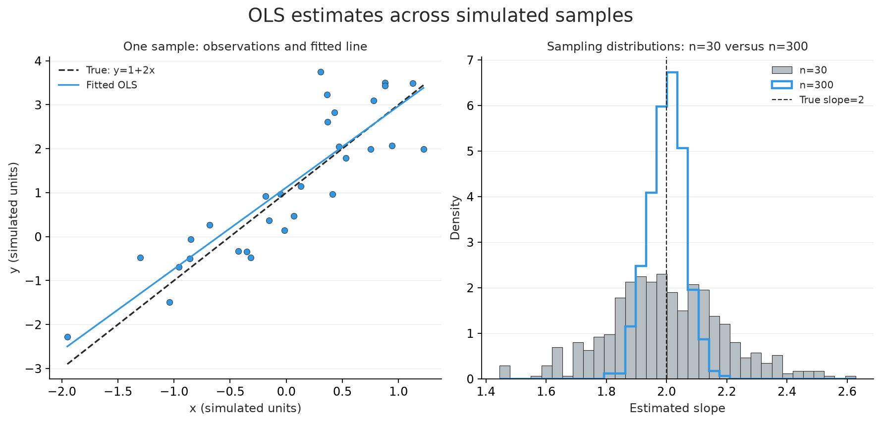
Figure 1: The left panel compares the true and fitted relationships in one sample; the right shows slope distributions across repeated samples. Larger samples produce a more concentrated distribution, while individual estimates can still depart from truth.

The slope means are approximately 1.997 and 2.001, with standard deviations 0.192 and 0.059. Both distributions centre near 2, but the larger sample varies less. This is more informative than showing one large-sample estimate closer to 2: sample size changes sampling behaviour without guaranteeing that every large sample outperforms every small one.

The same example supports further comparisons. What happens when error variance increases at fixed sample size? What if explanatory variables correlate with errors? The first concerns precision and the second model conditions. An editable calculation can distinguish greater dispersion from systematic deviation, and show why additional observations cannot automatically fix the latter.

Example two: interpreting regression coefficients

From a negative coefficient to an economic explanation

The first example supplied truth; the second uses observational data. Stata’s auto dataset contains 74 automobile models from 1978. Regressing price on fuel efficiency gives an mpg coefficient of approximately −238.89. Its direction prompts a useful question: why are more fuel-efficient models cheaper along this fitted relationship?

AI can run the regression in Stata and organise an interpretation around the negative coefficient:

Use Stata’s built-in auto data to run reg price mpg, preserving the original data file. Show the actual regression output and commands. Use the units of price and mpg to express the fitted relationship and compare fitted prices at 20 and 30 mpg. Develop possible economic explanations for why more fuel-efficient models have lower fitted prices, distinguishing what the regression supports from explanations that still need testing. Do not add other controls yet.

The output supports coefficient interpretation while retaining a baseline for later comparisons. This regression produces the following result:

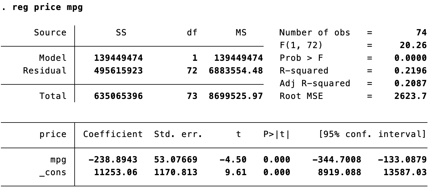
Figure 2: A simple automobile price–fuel-efficiency regression shows a negative relationship. The output supplies coefficients and uncertainty; interpreting that relationship requires considering other differences between models.

Reconstructing the fitted relationship turns the coefficient into a concrete comparison:

$$\widehat{\mathrm{price}}_i =11253.06-238.8943\,\mathrm{mpg}_i.$$

Price is in dollars and mpg in miles per gallon. A ten-unit increase along the fitted line corresponds to a price difference of about 2388.94 dollars. Fitted prices at 20 and 30 mpg are approximately 6475.17 and 4086.23 dollars. These points make the slope tangible but do not answer whether making the same car more fuel-efficient would reduce its price. The model compares different automobile models; weight, size, equipment and market positioning could relate to both price and efficiency.

How does a significant relationship become a supported explanation?

The interval of approximately $[-344.70,-133.09]$ supports a negative slope under the specified inference. Excluding zero does not select an economic mechanism. Smaller, lighter models might be more fuel-efficient and occupy different price segments, but this is a hypothesis to examine rather than a result already established by the regression.

The same question can guide further comparison: how does the mpg coefficient change after adding weight? If an added variable has missing values, have the included models changed too? Checking specification and effective sample together helps locate the source of coefficient changes. A control represents a justified comparison condition, not a way to decorate a regression table. Even with weight included, coefficient changes alone cannot establish causal identification.

The useful progression is from observing a negative coefficient to proposing an explanation and designing a comparison. Marx Max can retain the baseline code and output alongside subsequent calculations. Rather than restating every column’s definition, a teacher can ask students which claim the result supports, which needs further evidence and what the next regression is intended to test.

Example three: how MCMC approximates a posterior

Fixed data, a different object of sampling

Retain the first example’s 30 observations. Instead of regenerating data and examining estimator variation, infer parameters conditional on the observed data. To focus on MCMC, fix the intercept and error standard deviation and treat only the slope as unknown:

$$\begin{aligned} y_i&=1+\beta x_i+\varepsilon_i,\\ \varepsilon_i&\overset{\mathrm{iid}}{\sim}\mathcal{N}(0,1),\\ \beta&\sim\mathcal{N}(0,25). \end{aligned}$$

The prior variance is 25, giving standard deviation 5. Normal likelihood and prior yield an analytic posterior, providing a reference for MCMC. A solvable model isolates the algorithm: the target is known, so differences between finite sampling and that target can be examined directly.

Specify the model and comparison together so AI can generate the sampler and figure:

Reuse the first example’s 30 observations and use Python to compare random-walk Metropolis for one slope posterior. Fix the intercept and error standard deviation at 1 and use prior $\mathcal{N}(0,25)$ for the slope, where 25 is the variance. Derive the analytic posterior as a reference, then use proposal standard deviations 0.01, 0.35 and 3. Start each chain at 0 with seed 42, run 5000 iterations and retain the current state after rejections. Generate and run the code; plot full traces alongside densities of states retained after discarding the first 1000 iterations, in three rows and two columns. Overlay the analytic density and use common axes. Report acceptance rates and retained-state means and standard deviations.

The request specifies the statistical model separately from the algorithm comparison: the target stays fixed while proposal scale changes. The resulting figure supports a discussion of why three chains approaching the same target can give different finite-run results.

Define the target before interpreting sampling

The posterior is proportional to likelihood times prior. Ignoring constants independent of $\beta$, its log density is

$$\begin{aligned} \log p(\beta\mid x,y) &=-\frac{1}{2}\sum_{i=1}^{n}(y_i-1-\beta x_i)^2\\ &\quad-\frac{\beta^2}{2\cdot25}+C. \end{aligned}$$

Completing the square gives

$$\begin{aligned} V&=\left(\frac{1}{25}+\sum_{i=1}^{n}x_i^2\right)^{-1},\\ \mu&=V\sum_{i=1}^{n}x_i(y_i-1),\\ \beta\mid x,y&\sim\mathcal{N}(\mu,V). \end{aligned}$$

The posterior mean is approximately 1.853 and standard deviation 0.239. Unlike the first OLS fit, this model fixes the intercept and introduces a prior, so the means need not coincide. More fundamentally, this distribution concerns uncertainty conditional on these data and model, not a slope distribution across regenerated datasets. Both can appear as densities while answering different questions.

Why retain a state after rejection?

Symmetric normal random-walk Metropolis proposes a candidate from the current state and accepts according to the posterior-density ratio:

$$\beta^{\ast}=\beta_t+\eta_t,\qquad \eta_t\sim\mathcal{N}(0,s^2),$$ $$\alpha=\min\left\{1,\frac{p(\beta^{\ast}\mid x,y)} {p(\beta_t\mid x,y)}\right\}.$$

The proposal-density ratio cancels through symmetry, as does the target’s common normalising constant. Rejection leaves the next state at $\beta_t$, creating a horizontal trace segment. Retaining only accepted candidates discards holding times and changes the represented distribution. Repeated states therefore belong to the sample.

One posterior, three proposal scales

Hold data, prior and initial value 0 fixed and change only proposal standard deviation $s$ between 0.01, 0.35 and 3. Each chain runs for 5000 iterations. Right-hand densities use states after discarding the first 1000, compared with the analytic posterior.

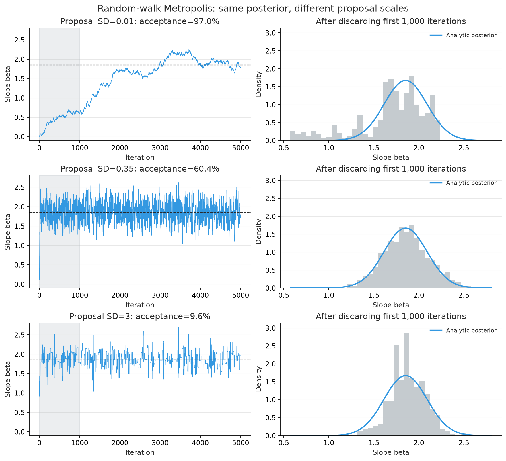
Figure 3: Small proposals are frequently accepted but explore slowly; large proposals often leave the chain stationary. The right panels compare retained-state densities with the blue analytic posterior, showing different exploration efficiency for one target.

Acceptance rates are approximately 97.0%, 60.4% and 9.6%. Despite its highest acceptance, the small-step chain has retained mean about 1.696, noticeably away from the analytic 1.853. Scale 0.35 gives mean 1.862 and standard deviation 0.252, closer to the reference. The large-step chain’s mean is 1.872 but standard deviation 0.199, differing from the target’s dispersion. Traces and distributions together reveal what an acceptance rate or a close mean alone cannot establish.

This separates target correctness from sufficient finite-chain exploration. Changing the prior changes the posterior target; changing proposal scale affects exploration efficiency. More iterations do not imply as many independent samples. Discarding 1000 states is a common comparison choice here, not proof of convergence. Formal work requires multiple chains and diagnostics such as effective sample size; see Stan’s posterior-analysis reference.

Connecting the examples

The examples develop three levels of understanding: OLS separates one estimate from sampling properties; automobile regression moves from a coefficient to an explanation and a testable comparison; MCMC distinguishes a statistical target from its computational approximation. Each requires a question, an explicit distinction between fixed and changed conditions, and an interpretation. Computation displays the differences; the reasoning supplies their teaching value.

Marx Max provides a shared, editable computation space for that work. Discussion stays alongside output, and changed conditions can be compared with earlier results. Developing one example before extending it helps preserve consistency between questions, models and interpretation.

Companion code

The Python example includes repeated OLS sampling, the analytic posterior and Metropolis, with a supplementary heteroskedasticity experiment. The Stata do-file reproduces the automobile regression. All simulations use seed 42 and the figures come from actual companion-code execution. Python needs NumPy and Matplotlib; Stata uses its built-in auto data. The do-file’s clear replaces in-memory data, so save existing work before reproducing it.