
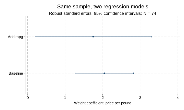
This case extends the guide’s first analysis: establish the data and sample, compare specifications, and retain reproducible code and outputs. The calculations below were actually executed in Stata using its bundled auto data. They illustrate model comparison, not a causal study of car prices.
Start with the Stata guide: connect, ask, and check output
Task and execution conditions
The calculation used Stata 19.5 without third-party commands. Both models use the same 74 observations with nonmissing price, weight and mpg and vce(robust). Readers with licensed Stata can rerun the program below. When using the request in Marx Max, check the code and output actually produced.
What did the two models produce?
| Model | Weight coefficient | Robust SE | 95% CI | N | R² |
|---|---|---|---|---|---|
| Weight only | 2.044 | 0.390 | 1.267–2.821 | 74 | 0.290 |
| Add mpg | 1.747 | 0.778 | 0.196–3.298 | 74 | 0.293 |
After adding mpg, the weight coefficient changes from about 2.044 to 1.747; the robust standard error and confidence interval become larger. Because the sample is fixed, this change is not due to excluded observations. The specification has changed, however: the second model is not automatically more correct, and neither establishes a causal effect of weight on price.
Download code and actual outputs
The package contains the complete do-file, actual run log, all model coefficients in CSV, SVG and PNG figures, and rerun instructions. It does not include Stata software or the source auto dataset.
- Download the do-file
- Download the coefficient table (CSV, readable in Excel)
- Read the actual run log
- View or save the vector figure (SVG)
How to rerun and check the results
- Extract into a fresh empty directory, separate from your research files.
- In a new Stata practice session, set the working directory to the extracted folder and run do analysis.do.
- Check the log for errors, confirm 74 observations and robust standard errors in both models, and compare the CSV coefficients and intervals.
- In Marx Max, first follow the guide to check the connection, then run the complete program in a new practice notebook. Retain code and output and investigate unexpected results from the actual log.
The program’s clear replaces data in memory; replace overwrites named outputs in the practice directory. Save current analyses first and use a new session and empty folder. This calculation ran in Stata 19.5 on macOS; rerunning on Windows hardware is not covered.
What to retain for your own research
Keep the sequence: define inputs and sample, execute specified models, inspect actual output, and save code and artifacts. Establish paths, variable meanings, controls, and standard errors for your research. Replacing auto with another file does not justify carrying over interpretations. Start with a bounded task and retain source material, reasons for changes, and the mapping from code to results.