
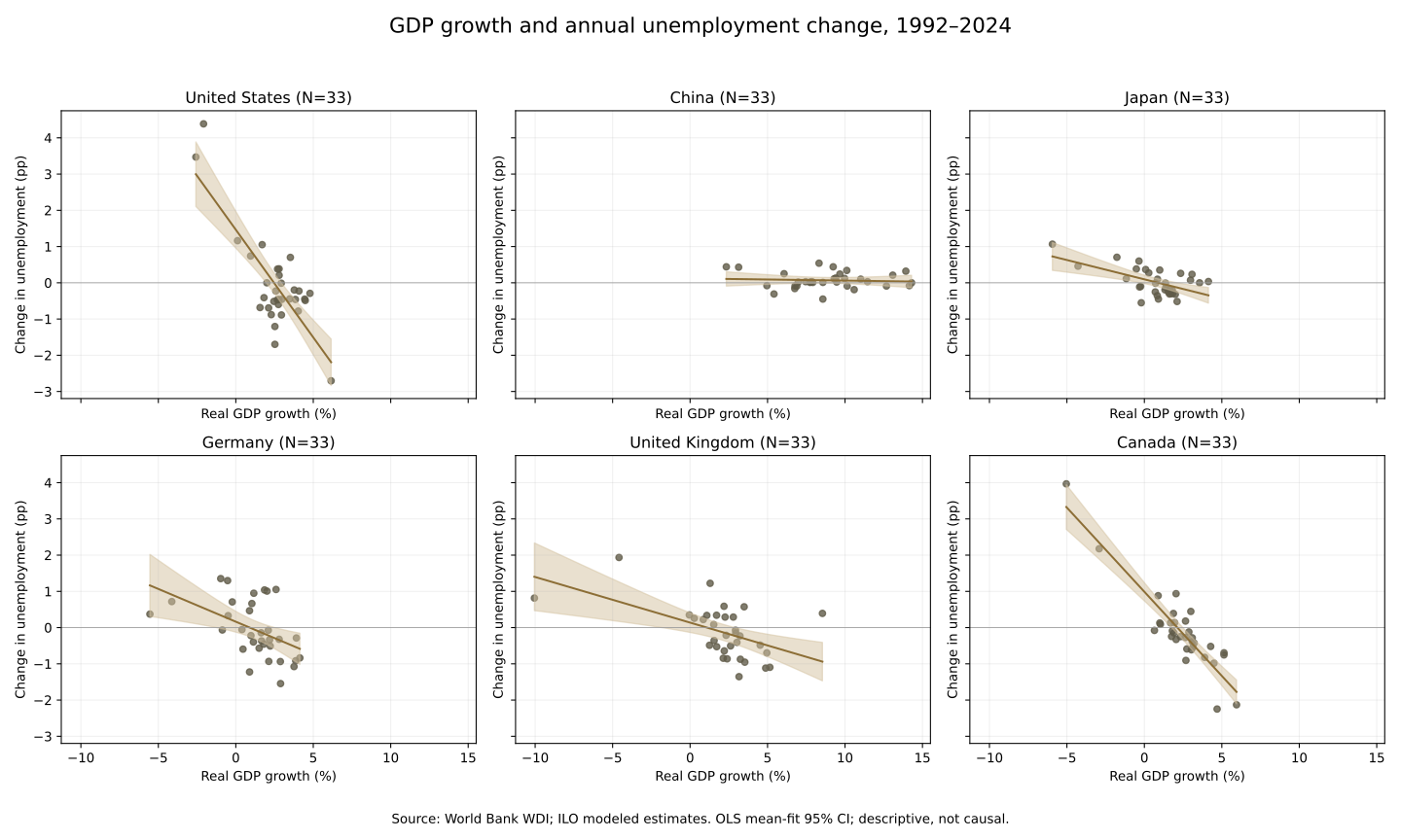
This case follows a public-data task from indicator definitions and source preservation to country/year alignment, unemployment changes, figures and regressions. Below are actual Python and Stata calculations on the same public-data snapshot, available to download and rerun independently.
Read the guide: define a public-data task and check artifacts
Starting point: two indicators and six countries
The task retains the original six countries: United States, China, Japan, Germany, United Kingdom and Canada, with annual data for 1991–2024. NY.GDP.MKTP.KD.ZG measures real GDP growth (%); SL.UEM.TOTL.ZS measures unemployment as a share of the labor force using ILO modeled estimates. This series includes modeled and imputed values and does not directly substitute for each country’s headline unemployment statistics.
- GDP definition, providers and license
- Unemployment definition, provider and limitations
- API URLs, retrieval time, data revision and hashes
The snapshot contains 204 country/year rows with no empty values in either indicator. The year 1991 supplies the lag for the first difference; plots and regressions use 1992–2024, with 33 observations per country. This exercise adds no imputation.
Processing: calculate changes, then fit each country separately
Annual unemployment change equals this year’s rate minus the previous year’s rate, in percentage points. GDP growth is on the horizontal axis and unemployment change on the vertical axis. Each country receives a separate OLS regression with an intercept. The programs check consecutive years rather than treating changes across gaps as annual differences or pooling all countries into one slope.
| Country | N | Slope | Conventional SE | 95% CI | R² |
|---|---|---|---|---|---|
| United States | 33 | -0.594 | 0.080 | -0.758–-0.431 | 0.640 |
| China | 33 | -0.006 | 0.014 | -0.034–0.022 | 0.006 |
| Japan | 33 | -0.107 | 0.027 | -0.162–-0.051 | 0.334 |
| Germany | 33 | -0.181 | 0.059 | -0.302–-0.060 | 0.230 |
| United Kingdom | 33 | -0.126 | 0.037 | -0.201–-0.051 | 0.276 |
| Canada | 33 | -0.464 | 0.039 | -0.544–-0.385 | 0.819 |
In this snapshot, the fitted negative slopes are more pronounced for the United States and Canada, while China’s fitted line is close to horizontal. The US slope of about −0.594 means a one-percentage-point difference in GDP growth corresponds to about −0.594 percentage points in annual unemployment change in this linear sample fit. It does not establish that increasing growth causes that change.
The exercise uses conventional OLS standard errors without adjustments for serial correlation, pandemic outliers or structural change. Figures and intervals are descriptive. The source warns about uncertainty in imputed values and their use for country rankings. Research requires additional checks on measurement, periods, lagged relationships and inference; six plots cannot establish a universal law.
Download: data, code, figures and actual output
The package includes raw API JSON, tidy CSV, provenance, separate Python and Stata programs, both sets of actual outputs and rerun instructions. Data are from World Bank WDI and its providers; both indicators specify CC BY 4.0. Attribution, modification notes and World Bank additional terms remain in the package. This exercise is not endorsed by the source institutions.
- Data CSV (readable in Excel)
- Country regression results CSV
- Actual Stata log
- PNG figure · Data attribution and terms · Complete rerun instructions
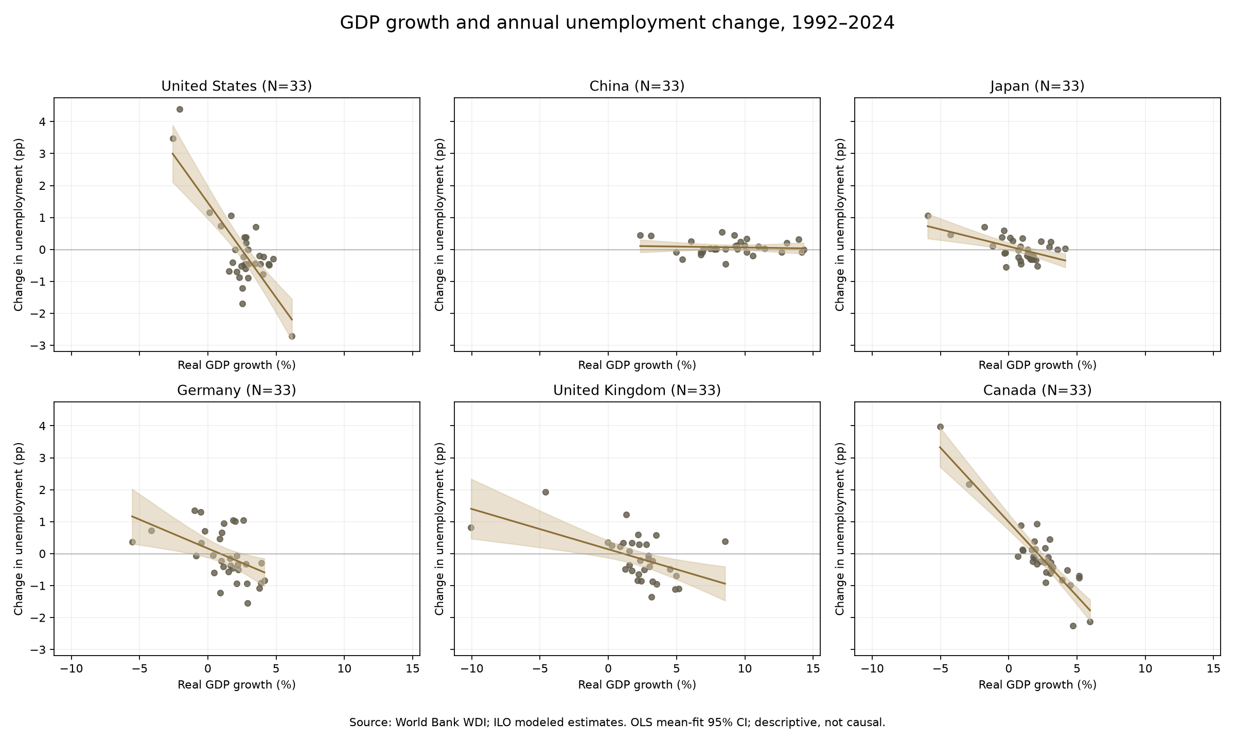
How to rerun
- Extract into a fresh empty directory and retain a reference copy of the outputs. The included data snapshot permits offline analysis without a World Bank account.
- For Python, prepare dependencies as described in the README and run python python/analyze.py from the package root. In a new licensed Stata session, change to the package root and run do stata/analysis.do; Python and third-party Stata commands are not required.
- Check six countries, 33 observations each, years 1992–2024, difference units and actual outputs. The two implementations were independently compared; maximum differences in coefficients, standard errors and intervals were below 10⁻¹⁰. Figure styles and file bytes need not match.
- For fresh data, copy the package separately, explicitly run python fetch-data.py and rerun analyses. Data revisions may change results; retain retrieval times and raw responses for comparisons.
Analysis programs overwrite named outputs in the practice directory, and Stata clear all clears that session’s memory state: save current work first. This run used macOS, Python 3.11.11 and Stata 19.5; Windows hardware reruns are not covered. In Marx Max, use a separate practice project and inspect actual code and output; cloud AI receives conversation and tool-returned content.
Return to the public-data guide · Understand AI data processing