
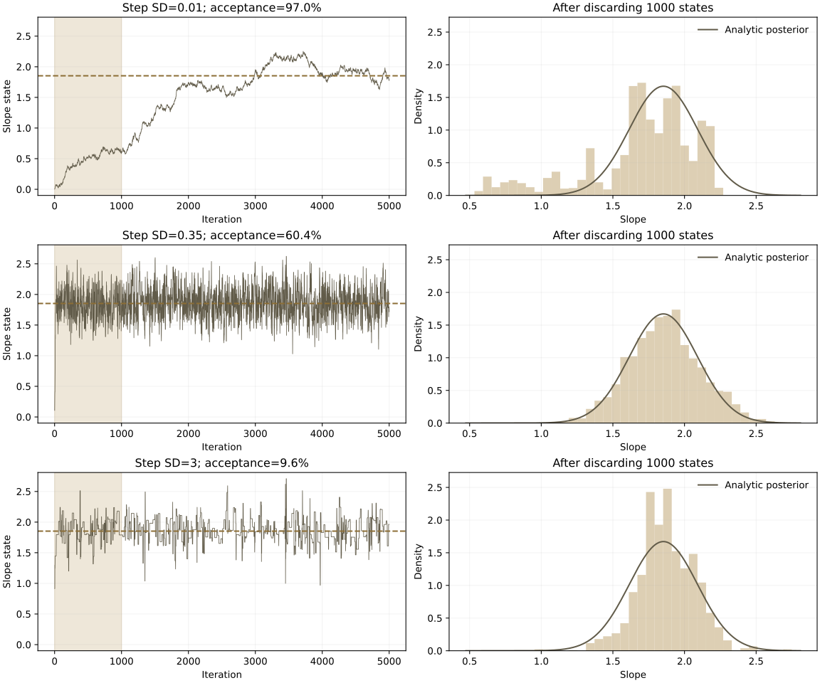
This case separates the statistical target from exploration by a finite chain. Data are entirely simulated and the target has an analytic reference. The executed program records every state and acceptance decision at three proposal scales.
Read the method and usage guide · Review OLS sampling distributions
Fix the data and posterior target first
Thirty simulated observations follow y=1+2x+ε with independent standard-normal x and ε, seed 42. Inference fixes intercept 1 and error SD 1, with slope prior N(0,5²). Only the slope is inferred, not intercept or variance. The analytic posterior mean is about 1.853 and SD 0.239.
Symmetric normal random-walk proposals have SD 0.01, 0.35 and 3, all starting at 0. Each setting runs 5,000 transitions and discards the first 1,000 states for comparison, retaining 4,000. Settings use the same seed and are not independent multiple chains for convergence diagnostics; they are not pooled into one posterior sample.
| Proposal SD | Full-run acceptance | Retained mean | Retained SD | Empirical 2.5%–97.5% quantiles |
|---|---|---|---|---|
| 0.01 | 97.0% | 1.696 | 0.381 | 0.683–2.187 |
| 0.35 | 60.4% | 1.862 | 0.252 | 1.381–2.362 |
| 3 | 9.6% | 1.872 | 0.199 | 1.465–2.236 |
The small scale accepts about 97%, but its retained mean of about 1.696 deviates from the analytic mean. The large scale accepts about 9.6% and often stays at one state. Scale 0.35 has mean and spread closer to the reference, but one run does not prove convergence. Acceptance covers all 5,000 transitions; other summaries use states after discarding 1,000.
Rejected proposals retain the previous state instead of exporting only accepted points. Discarding a prefix does not guarantee convergence, and empirical quantiles may be unreliable posterior intervals under poor exploration. Formal analysis needs appropriate independent chains and diagnostics such as effective sample size, which this exercise does not claim to provide. Stan posterior diagnostics
Download code, data and actual output
- Python
- Simulated input CSV · Results CSV · Every state and acceptance flag
- Actual Python output
- PNG · Dependencies, rerun and exercise instructions
- Extract into a fresh directory and retain reference outputs. Prepare Python dependencies following README. Installation accesses a package repository; analysis is offline.
- Run python analyze.py from the package root and check the completion marker, row counts and output. Defaults overwrite named files under the package results/.
- Use README commands to change seed or run length in a new output directory. Seed changes affect both data and proposal RNG; increasing iterations with the same seed keeps data and target fixed.
Runs used Python 3.11.11 on macOS; the heteroskedasticity case was independently checked in Stata 19.5. Windows hardware is not covered. Simulations illustrate methods and computation, not real research findings, classroom effects or automatic model performance.
Return to this case guide · Return to the econometrics teaching guide