
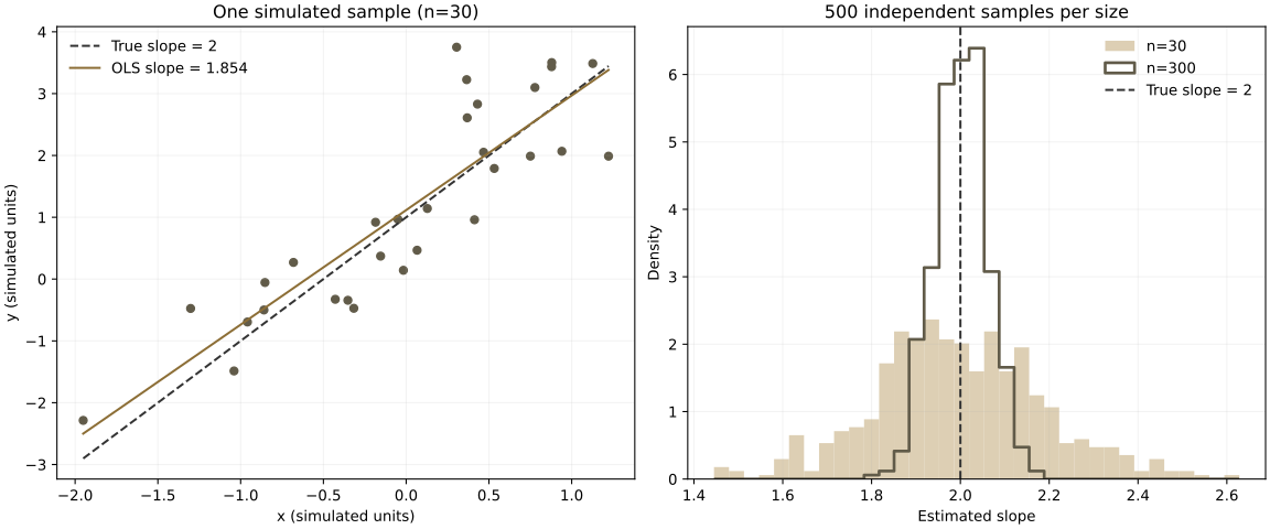
If the true slope is 2, why does one regression not return exactly 2? This teaching exercise uses entirely simulated data with a known truth to compare one estimate and repeated sampling. All figures and numbers come from the executed companion program, which you can rerun with another seed.
Read the econometrics teaching guide: OLS, coefficients and MCMC
What stays fixed, and what changes?
The generating model is y = 1 + 2x + ε. Both x and ε are independent standard normals, and observations are independent. The true intercept is 1 and slope is 2; the seed is 42. Draw 500 independent samples each at n=30 and n=300, displaying the first n=30 sample as a single OLS example. Smaller samples are not prefixes of the larger ones, and repeated regressions do not reuse one dataset.
One estimate and two sampling distributions
The single sample of 30 observations yields an intercept of about 1.116 and slope of about 1.854. Deviation from the truth alone does not establish a programming or model error. Check the program and then use repeated sampling to inspect variability.
| Sample size | Repetitions | Mean slope | SD of slopes | Empirical 2.5%–97.5% quantiles |
|---|---|---|---|---|
| 30 | 500 | 1.997 | 0.192 | 1.625–2.393 |
| 300 | 500 | 2.001 | 0.059 | 1.889–2.115 |
In this run, both means are close to 2 and the n=300 distribution is narrower. The SD describes variability across sampled coefficients, not the standard error reported by one regression; empirical quantiles are not that regression’s 95% confidence interval. Not every larger sample must yield an estimate closer to the truth.
The exercise assumes independent observations, homoskedastic errors and zero conditional error mean. Larger samples do not automatically repair endogeneity, measurement error or misspecification, and simulation does not establish identification assumptions in real research.
Download and rerun
- Python program
- 30 simulated observations (CSV) · 1,000 sampled slopes (CSV)
- Numerical summary · Actual run output · PNG
- Dependencies, rerun instructions and exercises
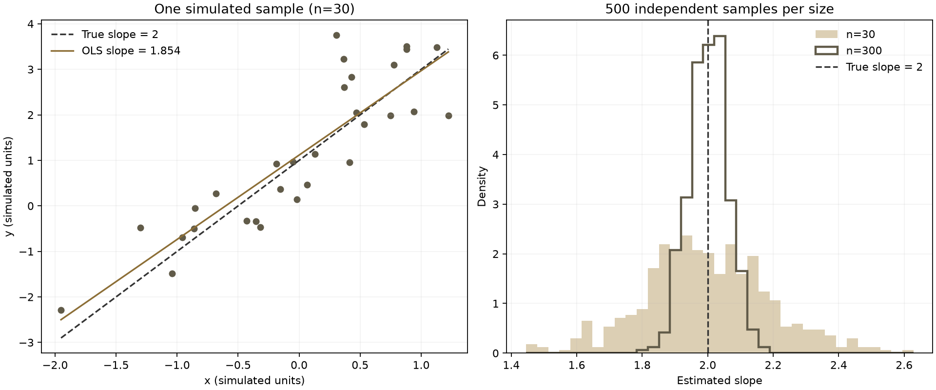
- Extract into a fresh practice directory and retain a reference copy. Follow the README to prepare Python, NumPy and Matplotlib. Installing dependencies accesses a package repository; analysis itself is offline.
- Run python analyze.py and check the completion marker, 30 single-sample rows, 1,000 slope rows and both summaries. The same parameters and dependency environment reproduce numbers; image bytes need not match.
- Change only the seed first, then increase repetitions, writing exercises to new directories. Compare individual estimates and distributions: more repetitions and more observations per sample are different changes.
The program only generates simulated data and overwrites named files under the package’s results/ by default. It was executed and rerun in a fresh directory on macOS with Python 3.11.11; Windows hardware is not covered. In Marx Max, use a separate project and discuss actual source and output. The package does not establish classroom learning effects or automatic model performance.
Return to the econometrics teaching guide · Continue to model comparison with actual Stata data