Robust standard errors

Open in Marx Max

Compare conventional and HC1 standard errors on 500 simulated observations with the same sample and coefficients. Download Python, Stata, simulated data, actual logs, figures and rerun instructions.

Use the public package’s 500 simulated observations, holding the sample and OLS coefficients fixed, to compare conventional and HC1 SEs, 95% intervals and p-values. Compute independently in Python and Stata, checking n/(n-k) with k=2 including the intercept and a t reference with 498 degrees of freedom. Read README.md, download into reference/ and retain original data and reference outputs. Check Python dependencies and licensed Stata, rerun in a fresh practice session and save current outputs and discrepancies into rerun/. Do not alter data to manufacture significance reversals, assume robust SEs are always larger, or treat HC1 as a cure for endogeneity or dependent errors.

OLS residuals and conventional versus HC1 standard errors on the same simulated sample. — Residual spread varies with x; the right panel compares intercept and slope SEs.

Download the complete rerun package (ZIP)

This case extends OLS sampling teaching by fixing data and regression while changing only the standard-error calculation. Data are entirely simulated and outputs independently calculated in Python and Stata for comparison.

Read the method and usage guide · Review OLS sampling distributions

One simulated sample; change only the covariance estimator

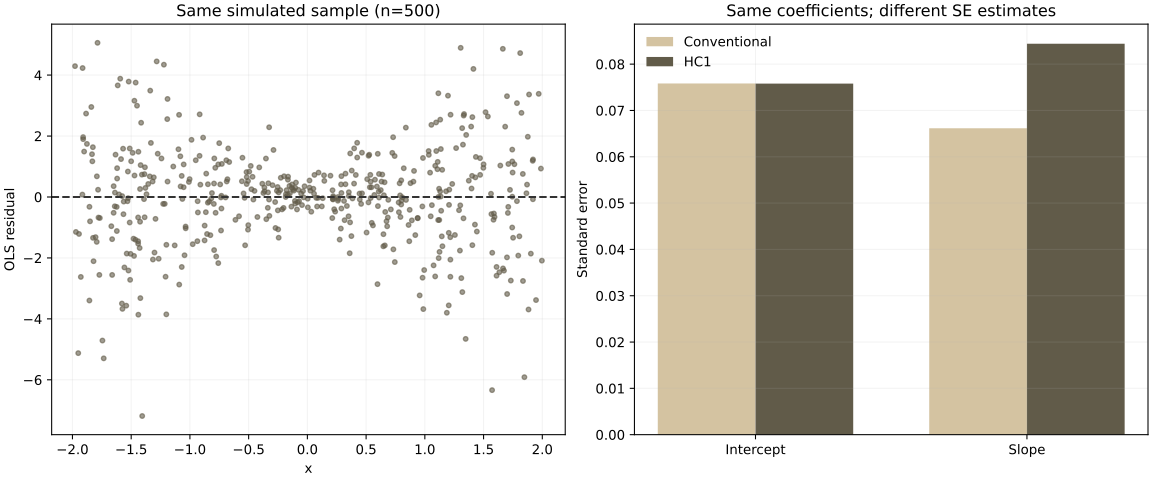
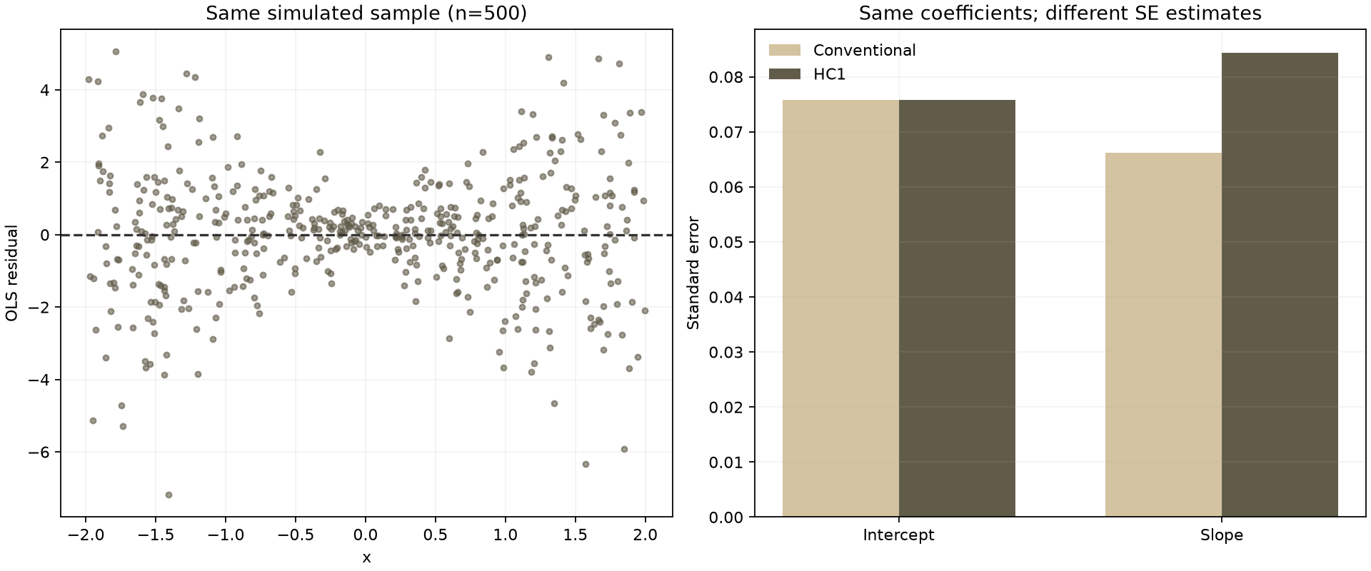
Seed 42 generates 500 independent observations. x is Uniform(−2,2) and z is independent standard normal; y = 1 + 2x + (0.3 + 1.2|x|)z. Errors have zero conditional mean and variance that depends on x. Both OLS fits include an intercept and all 500 rows, without sample or control changes.

Conventional covariance uses residual MSE. HC1 uses a residual-squared sandwich covariance with n/(n−k), where k=2 includes the intercept. Python computes the matrices explicitly; Stata uses regress y x and regress y x, vce(robust).

SE method	Slope	SE	95% interval	p	N
Conventional	1.973	0.066	1.843–2.103	7.65e-113	500
HC1	1.973	0.084	1.807–2.138	4.35e-82	500

The slope stays about 1.973 while its HC1 SE increases from about 0.066 to 0.084 and the interval widens. The intercept SEs are almost equal, with HC1 slightly smaller; full results are in CSV. The slope is significant under both reference calculations. This does not manufacture a significance reversal or imply robust SEs are always larger.

Intervals and p-values use a t reference with 498 degrees of freedom, not an exact finite-sample guarantee under heteroskedasticity. HC1 addresses the inference issue here, not endogeneity, omitted variables, within-group dependence or serial correlation. Official Stata methods

Download code, data and actual output

Extract into a fresh directory and retain reference outputs. Prepare Python dependencies following README. Installation accesses a package repository; analysis is offline.
Run python analyze.py from the package root and check the completion marker, row counts and output. Defaults overwrite named files under the package results/.
In a new licensed Stata session, change to the package root and run do analysis.do. Python and third-party Stata commands are not required. clear all clears session memory: save existing work first.

Runs used Python 3.11.11 on macOS; the heteroskedasticity case was independently checked in Stata 19.5. Windows hardware is not covered. Simulations illustrate methods and computation, not real research findings, classroom effects or automatic model performance.

Return to this case guide · Return to the econometrics teaching guide